Play Framework 2.5 | Dependency Injection 总结

最近在将Samsara Aquarius从Play 2.4.6迁移至Play 2.5.0的时候发现,Play 2.5将一些全局对象deprcated了,并强烈建议全面使用依赖注入来代替全局对象,所以就把Aquarius的代码用DI重构了一下。其实从Play 2.4.0开始就引入了依赖注入了(基于JSR 330标准),只不过还没有很好地推广。这里就来总结一下Play Framework中DI的使用。(本来开发的时候想保持FP风格的,无奈DI更多的是偏OO的风格。。FP与OO杂糅不好把握呀。。)

为何需要引入依赖注入

依赖注入(Dependency Injection)在OOP中早已是一个耳熟能详的原则了,其中Spring里用DI都用烂了。简单来说,依赖注入使得我们不需要自己创建对象,而是由容器来帮我们创建。每个组件之间不再是直接相互依赖,而是通过容器进行注入,这降低了组件之间的耦合度。这个容器就像是一个全局的大工厂,专门“生产”对象,而我们只需要进行配置(常见的通过XML文件或通过注解)。

在Play API中有一个Global对象,保存着一些全局的可变状态。另外还有一个Application对象相当于当前正在运行的Play实例。这两个伴生对象经常会在测试和部署的时候引发问题,并且也会影响Play实例的生命周期以及插件系统的工作。因此从Play 2.4开始,开发者对底层的结构做了很大的调整,底层所有的组件(包括Application、Route、Controller)都通过依赖注入进行管理,而不再使用Global和Application对象。后面版本中这两个对象只是从DI中获取实例的引用。从Play 2.5开始,这些全局对象被deprecated。

Play内部的DI组件都用的是 Google Guice。只要是符合JSR-330标准的DI组件都可用于Play Framework中。

DI in Play Framework

如何使用

比如我们的B组件需要A组件的实例作为依赖,我们可以这么定义:

1
2
3
import javax.inject.Inject
class B @Inject() (a: A)

注意,@Inject()需要插入在类名之后,构造参数列表之前,后边跟上需要注入的对象列表。

Guice里面的依赖注入有好几种方式构造注入方法注入 等等。这里采用最常用的构造注入。

生命周期及范围

依赖注入系统管理着各个注入组件的生命周期和范围。有以下规则:

  • 每次从Injector里取出的都是新的对象,即每次需要此组件的时候都会创建新的实例,用Spring IoC的话来说就是Bean的范围是 Prototype 。这一点和Spring不同(Spring默认是Singleton)。当然可以通过给待注入的类加上@Singleton注解来实现 Singleton
  • 遵循懒加载原则,即不用的时候就不创建。如果需要提前创建实例的话可以使用 Eager Binding

ApplicationLifecycle

有些组件需要在Play结束运行的时候进行一些清理工作,如关闭连接、关闭句柄。Play提供了ApplicationLifecycle类,可以通过addStopHook函数给组件注册回调,在Play结束运行的时候进行清理工作。addStopHook函数有两个版本,常用的是第一个:

1
2
3
def addStopHook(hook: () => Future[_]): Unit
def addStopHook(hook: Callable[_ <: CompletionStage[_]]): Unit

底层实现嘛比较直观,默认的实现是DefaultApplicationLifecycle类:

1
2
3
4
5
6
7
8
9
10
11
12
13
14
15
16
17
18
19
20
21
22
23
24
25
26
/**
* Default implementation of the application lifecycle.
*/
@Singleton
class DefaultApplicationLifecycle extends ApplicationLifecycle {
private val mutex = new Object()
@volatile private var hooks = List.empty[() => Future[_]]
def addStopHook(hook: () => Future[_]) = mutex.synchronized {
hooks = hook :: hooks
}
def stop(): Future[_] = {
// Do we care if one hook executes on another hooks redeeming thread? Hopefully not.
import play.api.libs.iteratee.Execution.Implicits.trampoline
hooks.foldLeft(Future.successful[Any](())) { (future, hook) =>
future.flatMap { _ =>
hook().recover {
case e => Logger.error("Error executing stop hook", e)
}
}
}
}
}

DefaultApplicationLifecycle类里维护了一个钩子列表hook用于存储所有注册的回调函数,类型为List[() => Future[_]]。由于DefaultApplicationLifecycle组件为单例,因此为避免资源争用,将hook变量声明为@volatile,并且注册回调函数时需要加锁。注意回调函数是按注册的顺序进行存储的。在应用结束时,会调用stop函数,通过foldLeft依次调用各个回调函数。

Play 应用重构实例

之前我把部分的Service设计成了Object(脑残了),并且在获取Slick的DatabaseConfig的时候使用了全局变量play.api.Play.current。这里我们来重构一下。

首先把Service重构为单例的类,并且通过DI的方式获取db。可以继承HasDatabaseConfigProvider[JdbcProfile]接口并注入DatabaseConfigProvider,这样Service就可以直接使用HasDatabaseConfigProviderdb对象了。当然如果不想继承HasDatabaseConfigProvider接口的话也可以仅注入DatabaseConfigProvider并自己在类中获取dbConfigdb(其它方式见Play-Slcik的文档)。

代码如下:

1
2
3
4
5
6
7
8
9
10
11
12
13
14
15
16
@Singleton
class UserService @Inject()(protected val dbConfigProvider: DatabaseConfigProvider) extends HasDatabaseConfigProvider[JdbcProfile] {
import driver.api._
private val users = TableQuery[UserTable]
def add(user: User): Future[Int] = {
db.run(users += user) recover {
case duplicate: com.mysql.jdbc.exceptions.MySQLIntegrityConstraintViolationException => DB_ADD_DUPLICATE
case _: Exception => -2
}
}
// 其他代码略......
}

接下来就是在Controller里配置DI将Service注入至Controller中。以UserController为例:

1
2
3
4
5
6
7
8
9
10
11
@Singleton
class UserController @Inject() (service: UserService) extends Controller {
def loginIndex = Action { implicit request =>
request.session.get("aq_token") match {
case Some(user) => Redirect(routes.Application.index())
case None => Ok(views.html.login(LoginForm.form))
}
} // 其他代码略......
}

DI底层调用过程

Play API中所有的DI都用的 Google Guice。它们最后都是调用了GuiceInjector类的instanceOf函数:

1
2
3
4
5
6
7
8
9
10
11
12
13
14
15
16
17
18
19
/**
* Play Injector backed by a Guice Injector.
*/
class GuiceInjector @Inject() (injector: com.google.inject.Injector) extends PlayInjector {
/**
* Get an instance of the given class from the injector.
*/
def instanceOf[T](implicit ct: ClassTag[T]) = instanceOf(ct.runtimeClass.asInstanceOf[Class[T]])
/**
* Get an instance of the given class from the injector.
*/
def instanceOf[T](clazz: Class[T]) = injector.getInstance(clazz)
/**
* Get an instance bound to the given binding key.
*/
def instanceOf[T](key: BindingKey[T]) = injector.getInstance(GuiceKey(key))
}

再往底层调用com.google.inject.internal#getProvider方法获取Provider,最终都会调用到某个种类的Injector的injectprovisionconstruct方法。

Call Stack

题外话-函数式编程中的DI

以前用DI的时候一直在想,这玩意在OOP中用途这么广泛,那么在FP里会是什么光景呢?其实在FP里,Currying 就可以当做是OOP中的DI。这里先挖个坑,待填坑:)

FP :: Type Theory | Type, Type Constructor 与 Kind

以前忘了总结了。。正好在这里总结一下 Type, Type ConstructorKind 这几个概念,结合Haskell和Scala。

TODO(2016.12): GHC 8.0的kind system(TypeInType); Dependent Type; Lambda Cube

Type, Type Constructor 与 Kind (Haskell)

Types and Programming Languages 里的一张图非常直观地表现了Kind与Type的意义:

其中,上图的Term就是值(Value)的意思,比如1"haha"之类的,都是Term。

而Type,则是 Value的类型,比如1的Type是Num(Haskell),"haha"的Type是String。然后我们引入Type Constructor的概念,它接受一个或多个类型参数(type parameter)并构造出一个新Type,比如Maybe是一个Unary Type Constructor,它接受一个类型参数,可以构造出Maybe IntMaybe String等等的不同的Type。再比如Either的定义为data Either a b = Left a | Right b,它接受两个类型参数,可以构造出像Either BoolEither Int Bool这样的Type Constructor。其实,我们也可以把这些Primitive Type看作是一种特殊的Type Constructor,即接受零个类型参数(Nullary Type Constructor)。

有了Type和Type Constructor的概念以后,我们就可以定义Kind了。Kind表示 Type Constructor的类型 ,在Haskell中有以下定义:

  • Nullary Type Constructor(即普通的Type)的kind为*
  • 如果k1和k2是kind,那么k1 -> k2代表一个Type constructor的kind,这个Constructor接受kind为k1的类型参数,返回kind为k2的类型参数。
    比如Either String的kind为* -> *

这样,从Value到Type、Type Constructor,再到Kind,每上一个层次都是一个抽象。Type Constructor是Value的类型,Kind又是Type Constructor的类型。

Kind Polymorphism (Haskell)

默认情况下,Haskell不允许kind具有多态性(Kind polymorphism)。比如我们的Either的定义如下:

1
data Either a b = Left a | Right b -- Defined in ‘Data.Either’

a和b的kind是任意的,可以是*,也可以是* -> *。Haskell默认将它们的kind都推导为*,因此下面的定义是不允许的:

1
2
3
4
5
6
7
8
Prelude> data T1 = Either []
<interactive>:123:18:
Expecting one more argument to ‘[]’
Expected a type, but ‘[]’ has kind ‘* -> *’
In the type ‘[]’
In the definition of data constructor ‘Either
In the data declaration for ‘T1

当然有些时候Haskell也是可以推导出来某些Higher-order kind的,比如:

1
data A t k p = A { s1 :: p, s2 :: t k }

由于s2 :: t k,而k默认被推导为*,因此t的kind就会被推导为* -> *,那么A的kind最终被推导为(* -> *) -> * -> * -> *

如果要使Haskell支持 polymorphic kinds ,可以利用GHC的扩展-XPolyKinds,就不再展开总结了,详情可以参考这里

Data Kinds/Datatype promotion (Haskell)

Datatype promotion是GHC的一个扩展(-XDataKinds),可以将部分的Datatype给自动promote成kind。比如:

1
2
3
4
5
6
7
8
Prelude> :k Left
Left :: k -> Either k k1
Prelude> :k 3
3 :: GHC.TypeLits.Nat
Prelude> :k ""
"" :: GHC.TypeLits.Symbol
Prelude> :k Just
Just :: k -> Maybe k

具体的应用还没实践过,等实践过再来总结。。

Scala中的Type和Kind

Scala中的Type和Kind用一张图总结:

我觉得Scala中的Kind比较混乱,至少每次试的时候出的结果总与想象的不对应,或许还没有理解吧。。。举几个例子:

1
2
3
4
5
6
7
8
9
10
11
12
13
14
15
16
17
18
19
20
21
22
23
24
25
26
27
28
29
30
31
32
33
34
35
36
37
scala> class Functor[M[_]]
defined class Functor
scala> :k -v Functor
<console>:11: error: not found: value Functor
Functor
^
scala> :k -v new Functor
Functor's kind is X[F[A]]
(* -> *) -> *
This is a type constructor that takes type constructor(s): a higher-kinded type.
scala> :k -v List
scala.collection.immutable.List's kind is F[+A]
* -(+)-> *
This is a type constructor: a 1st-order-kinded type.
scala> :k -v List[Int]
scala.collection.immutable.List's kind is F[+A]
* -(+)-> *
This is a type constructor: a 1st-order-kinded type.
scala> :k -v List(1, 2)
scala.collection.immutable.List's kind is A
*
This is a proper type.
scala> :k -v Either
scala.util.Either's kind is F[+A1,+A2]
* -(+)-> * -(+)-> *
This is a type constructor: a 1st-order-kinded type.
scala> :k -v (Int, String) => Option[_]
scala.Function2's kind is F[-A1,-A2,+A3]
* -(-)-> * -(-)-> * -(+)-> *
This is a type constructor: a 1st-order-kinded type.

感觉Scala REPL中的:kind是针对value的而不是type的,非常蛋疼,估计是让JVM的泛型类型擦除搞得Parametric Polymorphism都不爽了。。另外Scala中也分 1st-order-kinded typehigher-kinded type 。所谓higher-kinded type就是类似于A[B[_]]这样的type constructor,比如下面的这个例子:

1
2
3
4
5
6
7
8
9
10
11
12
13
14
15
scala> class T3[Q[A], P[B]]
defined class T3
scala> :k -v new T3
T3's kind is X[F1[A1],F2[A2]]
(* -> *) -> (* -> *) -> *
This is a type constructor that takes type constructor(s): a higher-kinded type.
scala> class T4[Tuple2[A, B], P[Option[C]], D, E]
defined class T4
scala> :k -v new T4
T4's kind is Y[F1[A1,A2],X[F2[A3]],A4,A5]
(* -> * -> *) -> ((* -> *) -> *) -> * -> * -> *
This is a type constructor that takes type constructor(s): a higher-kinded type.

参考资料

Scala | Haskell | Type Class总结

Type class in Haskell

Type class是Haskell中最重要的概念之一,它可以看做是 对一系列具有某种性质的type的抽象 (比如Eq, Functor, Monad之类的)。每个type class都定义了一组函数。一个type如果要成为某个type class,就必须成为其实例(instance)并实现type class定义的函数。表面上看起来type class和OOP中的接口(interface)的作用类似,但是type class有着更多的优点,我们将在后面比较type class与interface的特点。

在Haskell中,我们通过class关键字来定义type class。比如Monad的定义如下:

1
2
3
4
5
6
7
class Applicative m => Monad m where
(>>=) :: forall a b. m a -> (a -> m b) -> m b
(>>) :: forall a b. m a -> m b -> m b
return :: a -> m a
fail :: String -> m a

其中Applicative m => Monad m代表类型m(更严谨地说应该是type constructor,因为(m :: * -> *))同样是Applicative的实例。

我们可以通过instance关键字来实现type class的实例。比如Maybe Monad的实现如下:

1
2
3
4
5
6
7
8
9
10
data Maybe a = Nothing | Just a
deriving (Eq, Ord)
instance Monad Maybe where
(Just x) >>= k = k x
Nothing >>= _ = Nothing
(>>) = (*>)
fail _ = Nothing

Haskell引入type class是为了解决 Ad-hoc polymorphism 的问题。所谓的Ad-hoc polymorphism可以用一句话概括:

In programming languages, ad-hoc polymorphism is a kind of polymorphism in which polymorphic functions can be applied to arguments of different types, because a polymorphic function can denote a number of distinct and potentially heterogeneous implementations depending on the type of argument(s) to which it is applied.

即函数根据不同的参数类型选择不同版本的函数进行调用。Ad-hoc polymorphism在OOP里一般通过函数重载或运算符重载实现,而在Haskell中ad-hoc polymorphism就通过type class实现。比如show函数:

1
show :: Show a => a -> String

类型a必须是Show的实例,对于不同的类型ashow函数会选择对应的函数实现来进行调用,这就实现了上面所说的ad-hoc polymorphism(编译期):

1
2
3
4
5
6
Prelude> show [1.7, 6.4]
"[1.7,6.4]"
Prelude> show 2
"2"
Prelude> show $ Just 4
"Just 4"

Type class在Haskell中其实是一种语法糖,因此下面我们就来看一下GHC是如何desugar它的。

GHC处理type class的方式

我们来看一下GHC处理type class的方式。由于对于某个type,作用域内最多只能有一种某个type class的实例,因此type class可以被GHC处理成一种 “dictionary-passing style”。这里参考一下 A History of Haskell 中的例子:

1
2
3
4
5
6
7
8
9
10
11
12
13
14
15
16
17
class Eq a where
(==) :: a -> a -> Bool
(/=) :: a -> a -> Bool
instance Eq Int where
i1 == i2 = eqInt i1 i2
i1 /= i2 = not (i1 == i2)
instance (Eq a) => Eq [a] where
[] == [] = True
(x:xs) == (y:ys) = (x == y) && (xs == ys)
xs /= ys = not (xs == ys)
member :: Eq a => a -> [a] -> Bool
member x [] = False
member x (y:ys) | x == y = True
| otherwise = member x ys

它可以被转化成为以下形式:

1
2
3
4
5
6
7
8
9
10
11
12
13
14
15
16
17
18
data Eq a = MkEq (a -> a -> Bool) (a -> a -> Bool)
eq (MkEq e _) = e
ne (MkEq _ n) = n
dEqInt :: Eq Int
dEqInt = MkEq eqInt (\x y -> not (eqInt x y))
dEqList :: Eq a -> Eq [a]
dEqList d = MkEq el (\x y -> not (el x y))
where
el [] [] = True
el (x:xs) (y:ys) = eq d x y && el xs ys
el _ _ = False
member :: Eq a -> a -> [a] -> Bool
member d x [] = False
member d x (y:ys) | eq d x y = True
| otherwise = member d x ys

我们看到,type class的定义部分被转换成了一个data type,它定义了对应type class的字典(dictionary),里面记录了type class里的函数。上面的例子中,转换后的eqne函数会从这个字典里选择对应的函数。我们再来看一下转换后的member函数。它会接受对应的字典参数,并通过eq函数从字典中提取出对应的判断函数。最后就是对应的instance实现部分了。instance部分被转换成了一个选择函数,返回一个完整的字典。比如dEqList函数会接受一个Eq a类型的字典,返回一个Eq [a]类型的字典。

简单总结一下转换过程:

  • class -> data type (dictionary)
  • instance -> selector function

Type class pattern in Scala: Implicit Objects

Scala中并没有直接通过关键字支持type class(毕竟还混合了OOP)。Scala中type class成为了一种pattern,可以通过trait加上implicit来实现。

比如要对一组“可加的元素”(即我们熟悉的幺半群Monoid)进行求和(concat)操作,在Haskell里可以这么写(和默认的Monoid实现有差别):

1
2
3
4
5
6
7
8
9
10
11
12
13
14
15
16
{-# LANGUAGE FlexibleInstances #-}
class Monoid a where
mempty :: a
mappend :: a -> a -> a
instance Monoid Integer where
mempty = 0
mappend a b = a + b
instance Monoid String where
mempty = ""
mappend a b = a ++ b
mconcat :: Monoid a => [a] -> a
mconcat xs = foldl mappend mempty xs

而在Scala中,我们可以通过Implicit Object来实现:

1
2
3
4
5
6
7
8
9
10
11
12
13
14
15
16
17
18
trait Monoid[A] {
def mempty: A
def mappend(a: A, b: A): A
}
implicit object IntMonoid extends Monoid[Int] {
override def mempty = 0
override def mappend(a: Int, b: Int) = a + b
}
implicit object StringMonoid extends Monoid[String] {
override def mempty = ""
override def mappend(a: String, b: String) = a + b
}
def mconcat[A](xs: List[A])(implicit monoid: Monoid[A]): A = {
xs.foldLeft(monoid.mempty)(monoid.mappend)
}

首先我们定义了一个Monoid trait代表幺半群(性质:封闭、可结合、有幺元),这个trait就对应Haskell中type class的定义。接着我们分别为Int类型和String类型实现了对应的Monoid实例,注意对应的Monoid实例都是implicit object。最后我们要实现一个mconcat对一组具有幺半群性质的类型的值进行”求和”计算,这里我们将Monoid实例作为了implicit参数传递进了mconcat方法中,这样根据Scala的类型系统以及implicit匹配过程,当xs的类型是List[Int]的时候,IntMonoid会作为implicit参数传入mconcat方法;而当xs的类型是List[String]的时候,StringMonoid会作为implicit参数传入mconcat方法;如果没有匹配的implicit参数就会编译失败,从而确保了类型安全。是不是很奇妙呢?当然我们也可以用Scala的context bound语法糖省略掉implicit参数:

1
2
3
4
def mconcat[A : Monoid](xs: List[A]): A = {
val monoid = implicitly[Monoid[A]]
xs.foldLeft(monoid.mempty)(monoid.mappend)
}

Type class与接口的对比及优点

从上面的代码,我们可以看出,type class和trait/interface作用类似,都是对某一系列类型抽象出特定的行为。那么type class与trait/interface相比有什么优点呢?想象一下,如果用interface的话,每个sub-class都要在其body内实现对应的函数。这样如果要给现有的类实现这个interface的话,就必须要修改原类,在原类中增加对应的实现,这显然不符合Open Closed Principle(对扩展开放,对修改关闭)。所以OOP中提出了诸如 适配器模式 这样的设计模式用于扩展已有的类,但写各种adapter增加了代码的冗杂程度。

而对于type class pattern来说,实现type class实例的代码并不写在类型定义中,而是在外部实现一个对应type class的实例。这样,我们要给现有的类型实现一个type class的话就不需要更改原有类型的定义了,只需要实现对应的type class实例就可以了。这其实就是 抽象与实现分离,即类型定义与约束实现是分离的,某个类型并不清楚自己属于某个type class。与接口的方式相比,type class符合Open Closed Principle。

上面我们提到过,编译器会根据一定的机制在 编译期 自动寻找需要的type class实例,其中Haskell底层是通过转换成字典的形式让编译器寻找type class实例,而Scala中则是通过传入implicit参数的方式让编译器寻找type class实例,这保证了类型安全。

相比Haskell而言,Scala中的type class pattern更加灵活(托implicit的福),比如:

  • 结合context bound语法糖,Scala中可以方便的组合多个type class,如A : Eq : Ord
  • Type class可以有默认实现(default implicit parameter)
  • Scala中type class实例是具名的(implicit object),因此同一种类型可以有不同的type class实例,并且可以通过控制作用域(通过import)来选择不同的实例

当然type class还有更多的高级玩法,以后实践的多了再慢慢总结。。。


References

并发编程 | ThreadLocal 源码深入分析

以前只知道 ThreadLocal 的大致思路,没有去深入研究。今天读了读源码,果然博大精深~

ThreadLocal 提供了线程本地变量,它可以保证访问到的变量属于当前线程,每个线程都保存有一个变量副本,每个线程的变量都不同,而同一个线程在任何时候访问这个本地变量的结果都是一致的。当此线程结束生命周期时,所有的线程本地实例都会被 GC。ThreadLocal 相当于提供了一种线程隔离,将变量与线程相绑定。ThreadLocal 通常定义为 private static 类型。

假如让我们来实现一个变量与线程相绑定的功能,我们可以很容易地想到用HashMap来实现,Thread作为key,变量作为value。事实上,JDK 中确实使用了类似 Map 的结构存储变量,但不是像我们想的那样。下面我们来探究OpenJDK 1.8中ThreadLocal的实现。

初探 ThreadLocal

我们从 ThreadLocal 的几个成员变量入手:

1
2
3
4
5
6
7
8
9
10
11
12
13
14
15
16
17
18
19
20
21
22
private final int threadLocalHashCode = nextHashCode();
/**
* The next hash code to be given out. Updated atomically. Starts at
* zero.
*/
private static AtomicInteger nextHashCode =
new AtomicInteger();
/**
* The difference between successively generated hash codes - turns
* implicit sequential thread-local IDs into near-optimally spread
* multiplicative hash values for power-of-two-sized tables.
*/
private static final int HASH_INCREMENT = 0x61c88647;
/**
* Returns the next hash code.
*/
private static int nextHashCode() {
return nextHashCode.getAndAdd(HASH_INCREMENT);
}

ThreadLocal 通过 threadLocalHashCode 来标识每一个 ThreadLocal 的唯一性。threadLocalHashCode 通过 CAS 操作进行更新,每次 hash 操作的增量为 0x61c88647(这个数的原理没有探究)。

再看 set 方法:

1
2
3
4
5
6
7
8
9
10
11
12
13
14
15
16
17
/**
* Sets the current thread's copy of this thread-local variable
* to the specified value. Most subclasses will have no need to
* override this method, relying solely on the {@link #initialValue}
* method to set the values of thread-locals.
*
* @param value the value to be stored in the current thread's copy of
* this thread-local.
*/
public void set(T value) {
Thread t = Thread.currentThread();
ThreadLocalMap map = getMap(t);
if (map != null)
map.set(this, value);
else
createMap(t, value);
}

可以看到通过Thread.currentThread()方法获取了当前的线程引用,并传给了getMap(Thread)方法获取一个ThreadLocalMap的实例。我们继续跟进getMap(Thread)方法:

1
2
3
ThreadLocalMap getMap(Thread t) {
return t.threadLocals;
}

可以看到getMap(Thread)方法直接返回Thread实例的成员变量threadLocals。它的定义在Thread内部,访问级别为package级别:

1
2
3
/* ThreadLocal values pertaining to this thread. This map is maintained
* by the ThreadLocal class. */
ThreadLocal.ThreadLocalMap threadLocals = null;

到了这里,我们可以看出,每个Thread里面都有一个ThreadLocal.ThreadLocalMap成员变量,也就是说每个线程通过ThreadLocal.ThreadLocalMap与ThreadLocal相绑定,这样可以确保每个线程访问到的thread-local variable都是本线程的。

我们往下继续分析。获取了ThreadLocalMap实例以后,如果它不为空则调用ThreadLocalMap.ThreadLocalMap#set方法设值;若为空则调用ThreadLocal#createMap方法new一个ThreadLocalMap实例并赋给Thread.threadLocals

ThreadLocal#createMap方法的源码如下:

1
2
3
void createMap(Thread t, T firstValue) {
t.threadLocals = new ThreadLocalMap(this, firstValue);
}

下面我们探究一下 ThreadLocalMap 的实现。
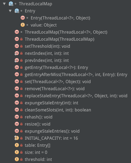
ThreadLocalMap

ThreadLocalMapThreadLocal 的静态内部类,它的结构如下:

ThreadLocalMap

可以看到ThreadLocalMap有一个常量和三个成员变量:

1
2
3
4
5
6
7
8
9
10
11
12
13
14
15
16
17
18
19
20
/**
* The initial capacity -- MUST be a power of two.
*/
private static final int INITIAL_CAPACITY = 16;
/**
* The table, resized as necessary.
* table.length MUST always be a power of two.
*/
private Entry[] table;
/**
* The number of entries in the table.
*/
private int size = 0;
/**
* The next size value at which to resize.
*/
private int threshold; // Default to 0

其中 INITIAL_CAPACITY代表这个Map的初始容量;table 是一个Entry 类型的数组,用于存储数据;size 代表表中的存储数目; threshold 代表需要扩容时对应 size 的阈值。

Entry 类是 ThreadLocalMap 的静态内部类,用于存储数据。它的源码如下:

1
2
3
4
5
6
7
8
9
10
11
12
13
14
15
16
17
/**
* The entries in this hash map extend WeakReference, using
* its main ref field as the key (which is always a
* ThreadLocal object). Note that null keys (i.e. entry.get()
* == null) mean that the key is no longer referenced, so the
* entry can be expunged from table. Such entries are referred to
* as "stale entries" in the code that follows.
*/
static class Entry extends WeakReference<ThreadLocal<?>> {
/** The value associated with this ThreadLocal. */
Object value;
Entry(ThreadLocal<?> k, Object v) {
super(k);
value = v;
}
}

Entry类继承了WeakReference<ThreadLocal<?>>,即每个Entry对象都有一个ThreadLocal的弱引用(作为key),这是为了防止内存泄露。一旦线程结束,key变为一个不可达的对象,这个Entry就可以被GC了。

ThreadLocalMap类有两个构造函数,其中常用的是ThreadLocalMap(ThreadLocal<?> firstKey, Object firstValue)

1
2
3
4
5
6
7
8
9
10
11
12
/**
* Construct a new map initially containing (firstKey, firstValue).
* ThreadLocalMaps are constructed lazily, so we only create
* one when we have at least one entry to put in it.
*/
ThreadLocalMap(ThreadLocal<?> firstKey, Object firstValue) {
table = new Entry[INITIAL_CAPACITY];
int i = firstKey.threadLocalHashCode & (INITIAL_CAPACITY - 1);
table[i] = new Entry(firstKey, firstValue);
size = 1;
setThreshold(INITIAL_CAPACITY);
}

构造函数的第一个参数就是本ThreadLocal实例(this),第二个参数就是要保存的线程本地变量。构造函数首先创建一个长度为16的Entry数组,然后计算出firstKey对应的哈希值,然后存储到table中,并设置size和threshold。

注意一个细节,计算hash的时候里面采用了hashCode & (size - 1)的算法,这相当于取模运算hashCode % size的一个更高效的实现(和HashMap中的思路相同)。正是因为这种算法,我们要求size必须是 2的指数,因为这可以使得hash发生冲突的次数减小。

接下来我们来看ThreadLocalMap#set方法的实现:

1
2
3
4
5
6
7
8
9
10
11
12
13
14
15
16
17
18
19
20
21
22
23
24
25
26
27
28
29
30
31
32
33
34
35
36
37
38
/**
* Set the value associated with key.
*
* @param key the thread local object
* @param value the value to be set
*/
private void set(ThreadLocal<?> key, Object value) {
// We don't use a fast path as with get() because it is at
// least as common to use set() to create new entries as
// it is to replace existing ones, in which case, a fast
// path would fail more often than not.
Entry[] tab = table;
int len = tab.length;
int i = key.threadLocalHashCode & (len-1);
for (Entry e = tab[i];
e != null;
e = tab[i = nextIndex(i, len)]) {
ThreadLocal<?> k = e.get();
if (k == key) {
e.value = value;
return;
}
if (k == null) {
replaceStaleEntry(key, value, i);
return;
}
}
tab[i] = new Entry(key, value);
int sz = ++size;
if (!cleanSomeSlots(i, sz) && sz >= threshold)
rehash();
}

如果冲突了,就会通过nextIndex方法再次计算哈希值:

1
2
3
4
5
6
/**
* Increment i modulo len.
*/
private static int nextIndex(int i, int len) {
return ((i + 1 < len) ? i + 1 : 0);
}

到这里,我们看到 ThreadLocalMap 解决冲突的方法是 线性探测法(不断加 1),而不是 HashMap 的 链地址法,这一点也能从 Entry 的结构上推断出来。

如果entry里对应的key为null的话,表明此entry为staled entry,就将其替换为当前的key和value:

1
2
3
4
5
6
7
8
9
10
11
12
13
14
15
16
17
18
19
20
21
22
23
24
25
26
27
28
29
30
31
32
33
34
35
36
37
38
39
40
41
42
43
44
45
46
47
48
49
50
51
52
53
54
55
56
57
58
59
60
61
62
63
64
65
66
67
68
69
70
71
72
/**
* Replace a stale entry encountered during a set operation
* with an entry for the specified key. The value passed in
* the value parameter is stored in the entry, whether or not
* an entry already exists for the specified key.
*
* As a side effect, this method expunges all stale entries in the
* "run" containing the stale entry. (A run is a sequence of entries
* between two null slots.)
*
* @param key the key
* @param value the value to be associated with key
* @param staleSlot index of the first stale entry encountered while
* searching for key.
*/
private void replaceStaleEntry(ThreadLocal<?> key, Object value,
int staleSlot) {
Entry[] tab = table;
int len = tab.length;
Entry e;
// Back up to check for prior stale entry in current run.
// We clean out whole runs at a time to avoid continual
// incremental rehashing due to garbage collector freeing
// up refs in bunches (i.e., whenever the collector runs).
int slotToExpunge = staleSlot;
for (int i = prevIndex(staleSlot, len);
(e = tab[i]) != null;
i = prevIndex(i, len))
if (e.get() == null)
slotToExpunge = i;
// Find either the key or trailing null slot of run, whichever
// occurs first
for (int i = nextIndex(staleSlot, len);
(e = tab[i]) != null;
i = nextIndex(i, len)) {
ThreadLocal<?> k = e.get();
// If we find key, then we need to swap it
// with the stale entry to maintain hash table order.
// The newly stale slot, or any other stale slot
// encountered above it, can then be sent to expungeStaleEntry
// to remove or rehash all of the other entries in run.
if (k == key) {
e.value = value;
tab[i] = tab[staleSlot];
tab[staleSlot] = e;
// Start expunge at preceding stale entry if it exists
if (slotToExpunge == staleSlot)
slotToExpunge = i;
cleanSomeSlots(expungeStaleEntry(slotToExpunge), len);
return;
}
// If we didn't find stale entry on backward scan, the
// first stale entry seen while scanning for key is the
// first still present in the run.
if (k == null && slotToExpunge == staleSlot)
slotToExpunge = i;
}
// If key not found, put new entry in stale slot
tab[staleSlot].value = null;
tab[staleSlot] = new Entry(key, value);
// If there are any other stale entries in run, expunge them
if (slotToExpunge != staleSlot)
cleanSomeSlots(expungeStaleEntry(slotToExpunge), len);
}

具体实现不再深究,这替换过程里面也进行了不少的垃圾清理动作以防止引用关系存在而导致的内存泄露。

若是经历了上面步骤没有命中hash,也没有发现无用的Entry,set方法就会创建一个新的Entry,并会进行启发式的垃圾清理,用于清理无用的Entry。主要通过cleanSomeSlots方法进行清理(清理的时机通常为添加新元素或另一个无用的元素被回收时。参见注释):

1
2
3
4
5
6
7
8
9
10
11
12
13
14
15
16
17
18
19
20
21
22
23
24
25
26
27
28
29
30
31
32
33
34
35
36
37
38
39
/**
* Heuristically scan some cells looking for stale entries.
* This is invoked when either a new element is added, or
* another stale one has been expunged. It performs a
* logarithmic number of scans, as a balance between no
* scanning (fast but retains garbage) and a number of scans
* proportional to number of elements, that would find all
* garbage but would cause some insertions to take O(n) time.
*
* @param i a position known NOT to hold a stale entry. The
* scan starts at the element after i.
*
* @param n scan control: {@code log2(n)} cells are scanned,
* unless a stale entry is found, in which case
* {@code log2(table.length)-1} additional cells are scanned.
* When called from insertions, this parameter is the number
* of elements, but when from replaceStaleEntry, it is the
* table length. (Note: all this could be changed to be either
* more or less aggressive by weighting n instead of just
* using straight log n. But this version is simple, fast, and
* seems to work well.)
*
* @return true if any stale entries have been removed.
*/
private boolean cleanSomeSlots(int i, int n) {
boolean removed = false;
Entry[] tab = table;
int len = tab.length;
do {
i = nextIndex(i, len);
Entry e = tab[i];
if (e != null && e.get() == null) {
n = len;
removed = true;
i = expungeStaleEntry(i);
}
} while ( (n >>>= 1) != 0);
return removed;
}

一旦发现一个位置对应的 Entry 所持有的 ThreadLocal 弱引用为null,就会把此位置当做 staleSlot 并调用 expungeStaleEntry 方法进行整理 (rehashing) 的操作:

1
2
3
4
5
6
7
8
9
10
11
12
13
14
15
16
17
18
19
20
21
22
23
24
25
26
27
28
29
30
31
32
33
34
35
36
37
38
39
40
41
42
43
44
45
46
/**
* Expunge a stale entry by rehashing any possibly colliding entries
* lying between staleSlot and the next null slot. This also expunges
* any other stale entries encountered before the trailing null. See
* Knuth, Section 6.4
*
* @param staleSlot index of slot known to have null key
* @return the index of the next null slot after staleSlot
* (all between staleSlot and this slot will have been checked
* for expunging).
*/
private int expungeStaleEntry(int staleSlot) {
Entry[] tab = table;
int len = tab.length;
// expunge entry at staleSlot
tab[staleSlot].value = null;
tab[staleSlot] = null;
size--;
// Rehash until we encounter null
Entry e;
int i;
for (i = nextIndex(staleSlot, len);
(e = tab[i]) != null;
i = nextIndex(i, len)) {
ThreadLocal<?> k = e.get();
if (k == null) {
e.value = null;
tab[i] = null;
size--;
} else {
int h = k.threadLocalHashCode & (len - 1);
if (h != i) {
tab[i] = null;
// Unlike Knuth 6.4 Algorithm R, we must scan until
// null because multiple entries could have been stale.
while (tab[h] != null)
h = nextIndex(h, len);
tab[h] = e;
}
}
}
return i;
}

只要没有清理任何的 stale entries 并且 size 达到阈值的时候(即 table 已满,所有元素都可用),都会触发rehashing

1
2
3
4
5
6
7
8
9
10
11
12
13
14
15
16
17
18
19
20
21
22
23
24
25
/**
* Re-pack and/or re-size the table. First scan the entire
* table removing stale entries. If this doesn't sufficiently
* shrink the size of the table, double the table size.
*/
private void rehash() {
expungeStaleEntries();
// Use lower threshold for doubling to avoid hysteresis
if (size >= threshold - threshold / 4)
resize();
}
/**
* Expunge all stale entries in the table.
*/
private void expungeStaleEntries() {
Entry[] tab = table;
int len = tab.length;
for (int j = 0; j < len; j++) {
Entry e = tab[j];
if (e != null && e.get() == null)
expungeStaleEntry(j);
}
}

rehash 操作会执行一次全表的扫描清理工作,并在 size 大于等于 threshold 的四分之三时进行 resize。但注意在 setThreshold 的时候又取了三分之二:

1
2
3
4
5
6
/**
* Set the resize threshold to maintain at worst a 2/3 load factor.
*/
private void setThreshold(int len) {
threshold = len * 2 / 3;
}

因此 ThreadLocalMap 的实际 load factor 为 3/4 * 2/3 = 0.5

我们继续看 getEntry 的源码:

1
2
3
4
5
6
7
8
9
10
11
12
13
14
15
16
17
18
19
20
21
22
23
24
25
26
27
28
29
30
31
32
33
34
35
36
37
38
39
40
41
42
43
44
/**
* Get the entry associated with key. This method
* itself handles only the fast path: a direct hit of existing
* key. It otherwise relays to getEntryAfterMiss. This is
* designed to maximize performance for direct hits, in part
* by making this method readily inlinable.
*
* @param key the thread local object
* @return the entry associated with key, or null if no such
*/
private Entry getEntry(ThreadLocal<?> key) {
int i = key.threadLocalHashCode & (table.length - 1);
Entry e = table[i];
if (e != null && e.get() == key)
return e;
else
return getEntryAfterMiss(key, i, e);
}
/**
* Version of getEntry method for use when key is not found in
* its direct hash slot.
*
* @param key the thread local object
* @param i the table index for key's hash code
* @param e the entry at table[i]
* @return the entry associated with key, or null if no such
*/
private Entry getEntryAfterMiss(ThreadLocal<?> key, int i, Entry e) {
Entry[] tab = table;
int len = tab.length;
while (e != null) {
ThreadLocal<?> k = e.get();
if (k == key)
return e;
if (k == null)
expungeStaleEntry(i);
else
i = nextIndex(i, len);
e = tab[i];
}
return null;
}

逻辑很简单,hash以后如果是ThreadLocal对应的Entry就返回,否则调用getEntryAfterMiss方法,根据线性探测法继续查找,直到找到或对应entry为null,并返回。

ThreadLocal的get方法就是调用了ThreadLocalMap的getEntry方法:

1
2
3
4
5
6
7
8
9
10
11
12
13
public T get() {
Thread t = Thread.currentThread();
ThreadLocalMap map = getMap(t);
if (map != null) {
ThreadLocalMap.Entry e = map.getEntry(this);
if (e != null) {
@SuppressWarnings("unchecked")
T result = (T)e.value;
return result;
}
}
return setInitialValue();
}

remove 方法的思想类似,直接放源码:

1
2
3
4
5
6
7
8
9
10
11
12
13
14
15
16
17
/**
* Remove the entry for key.
*/
private void remove(ThreadLocal<?> key) {
Entry[] tab = table;
int len = tab.length;
int i = key.threadLocalHashCode & (len-1);
for (Entry e = tab[i];
e != null;
e = tab[i = nextIndex(i, len)]) {
if (e.get() == key) {
e.clear();
expungeStaleEntry(i);
return;
}
}
}

remove的时候同样也会调用expungeStaleEntry方法执行清理工作。

总结

每个 Thread 里都含有一个 ThreadLocalMap 的成员变量,这种机制将 ThreadLocal 和线程巧妙地绑定在了一起,即可以保证无用的 ThreadLocal 被及时回收,不会造成内存泄露,又可以提升性能。假如我们把 ThreadLocalMap 做成一个 Map<t extends Thread, ?> 类型的 Map,那么它存储的东西将会非常多(相当于一张全局线程本地变量表),这样的情况下用线性探测法解决哈希冲突的问题效率会非常差。而 JDK 里的这种利用 ThreadLocal 作为 key,再将 ThreadLocalMap 与线程相绑定的实现,完美地解决了这个问题。

总结一下什么时候无用的 Entry 会被清理:

  • Thread 结束的时候
  • 插入元素时,发现 staled entry,则会进行替换并清理
  • 插入元素时,ThreadLocalMapsize 达到 threshold,并且没有任何 staled entries 的时候,会调用 rehash 方法清理并扩容
  • 调用 ThreadLocalMapremove 方法或set(null)

尽管不会造成内存泄露,但是可以看到无用的 Entry 只会在以上四种情况下才会被清理,这就可能导致一些 Entry 虽然无用但还占内存的情况。因此,我们在使用完 ThreadLocal 后一定要remove一下,保证及时回收掉无用的 Entry。

特别地,当应用线程池的时候,由于线程池的线程一般会复用,Thread 不结束,这时候用完更需要 remove 了。

总的来说,对于多线程资源共享的问题,同步机制采用了 以时间换空间 的方式,而 ThreadLocal 则采用了 以空间换时间 的方式。前者仅提供一份变量,让不同的线程排队访问;而后者为每一个线程都提供了一份变量,因此可以同时访问而互不影响。

应用

应用太多了,举个 Spring 的例子。Spring 对一些 Bean 中的成员变量采用 ThreadLocal 进行处理,让它们可以成为线程安全的。举个例子:

1
2
3
4
5
6
7
8
9
10
11
12
13
14
15
package org.springframework.web.context.request;
public abstract class RequestContextHolder {
private static final boolean jsfPresent =
ClassUtils.isPresent("javax.faces.context.FacesContext", RequestContextHolder.class.getClassLoader());
private static final ThreadLocal<RequestAttributes> requestAttributesHolder =
new NamedThreadLocal<RequestAttributes>("Request attributes");
private static final ThreadLocal<RequestAttributes> inheritableRequestAttributesHolder =
new NamedInheritableThreadLocal<RequestAttributes>("Request context");
//......下面省略
}

再比如 Spring MVC 中的 Controller 默认是 singleton 的,因此如果 Controller 或其对应的 Service 里存在非静态成员变量的话,并发访问就会出现 race condition 问题,这也可以通过 ThreadLocal 解决。

并发编程 | JDK 1.8 中的 CompletableFuture | FRP风格

在异步编程中,Future/Promise模式是一种广泛使用的异步开发模式,其中 Future 对象代表一个尚未完成异步操作的结果。从JDK 1.5以来,JUC包一直提供着最基本的Future,不过它太鸡肋了,除了getcancelisDoneisCancelled方法之外就没有其他的操作了,这样很不方便。好在JDK 1.8中引入了具有FRP风格的 CompletableFuture,它类似于Scala中的 FutureCompletableFuture 属于Monad, 因此支持一系列的函数式的组合、运算操作,非常方便,可以写出很FRP风格的代码而摆脱callback hell。

下面我们来结合FRP的思想,总结一下这些操作(有的时候为了方便表示,我会用Haskell或Scala的语法来表示类型,毕竟Java的类型系统太渣):

构造CompletableFuture对象

CompletableFuture类通过工厂模式创建CompletableFuture对象:

1
2
3
4
5
6
7
8
9
10
11
12
13
14
15
16
17
public static <U> CompletableFuture<U> supplyAsync(Supplier<U> supplier) {
return asyncSupplyStage(asyncPool, supplier);
}
public static <U> CompletableFuture<U> supplyAsync(Supplier<U> supplier,
Executor executor) {
return asyncSupplyStage(screenExecutor(executor), supplier);
}
public static CompletableFuture<Void> runAsync(Runnable runnable) {
return asyncRunStage(asyncPool, runnable);
}
public static CompletableFuture<Void> runAsync(Runnable runnable,
Executor executor) {
return asyncRunStage(screenExecutor(executor), runnable);
}

如果我们的异步操作不需要返回值,那么可以通过runAsync方法提供一个Runnable创建一个CompletableFuture<Void>对象。如果我们的异步操作需要返回值,那么可以通过supplyAsync方法提供一个Supplier<U>对象来创建:

1
final CompletableFuture<String> future = CompletableFuture.supplyAsync(() -> longTask(param));

如果不提供Executor的话,默认使用ForkJoinPool.commonPool()作为线程池。

后缀为Async的方法代表异步执行。

变换(fmap)

假如我们要通过CompletableFuture来异步获取一组数据,并对数据进行一些处理(变换),我们可以使用thenApplythenApplyAsync方法:

1
2
3
4
5
6
7
8
9
10
11
12
13
14
public <U> CompletableFuture<U> thenApply(
Function<? super T,? extends U> fn) {
return uniApplyStage(null, fn);
}
public <U> CompletableFuture<U> thenApplyAsync(
Function<? super T,? extends U> fn) {
return uniApplyStage(asyncPool, fn);
}
public <U> CompletableFuture<U> thenApplyAsync(
Function<? super T,? extends U> fn, Executor executor) {
return uniApplyStage(screenExecutor(executor), fn);
}

它其实就是fmap函数,用Haskell表示原型为:

1
2
3
4
-- 对比一下fmap
fmap :: Functor f => (a -> b) -> f a -> f b
thenApply :: (a -> b) -> CompletableFuture a -> CompletableFuture b

它们不仅可以变换数据的值,也可以变换数据的类型,如:

1
2
3
CompletableFuture<Double> f = CompletableFuture.supplyAsync(() -> "4")
.thenApply(Integer::parseInt)
.thenApply(r -> r * r * Math.PI);

fmap以后,数据流的类型进行了以下变换:String -> Integer -> Double

组合(bind)

有的时候,我们需要在异步操作完成的时候对异步操作的结果进行一些操作,并且操作仍然返回CompletableFuture类型。我们可以利用thenCompose方法:

1
2
3
4
5
6
7
8
9
10
11
12
13
14
15
public <U> CompletableFuture<U> thenCompose(
Function<? super T, ? extends CompletionStage<U>> fn) {
return uniComposeStage(null, fn);
}
public <U> CompletableFuture<U> thenComposeAsync(
Function<? super T, ? extends CompletionStage<U>> fn) {
return uniComposeStage(asyncPool, fn);
}
public <U> CompletableFuture<U> thenComposeAsync(
Function<? super T, ? extends CompletionStage<U>> fn,
Executor executor) {
return uniComposeStage(screenExecutor(executor), fn);
}

可以看出它其实对应了Monad里的bind操作(Java和Scala中为flatMap),用Haskell表示原型为:

1
2
3
(>>=) :: Monad m => m a -> (a -> m b) -> m b
thenCompose :: CompletableFuture a -> (a -> CompletableFuture b) -> CompletableFuture b

thenCompose是一个非常重要的操作,它对于构建异步的pipeline非常有用。举个简单的例子:

1
2
3
4
5
6
7
8
9
10
11
12
13
14
15
16
17
18
19
20
21
22
23
24
25
26
27
28
29
30
31
public class TaskWorkI {
public static Optional<List<Integer>> longTask(Integer i) {
if (i > 0) {
List<Integer> list = new ArrayList<>();
for(int pc = 0; pc < i; pc++)
list.add(pc);
return Optional.of(list);
}
else
return Optional.empty();
}
public static CompletableFuture<Long> getResultFuture(Optional<List<Integer>> op) {
return CompletableFuture.supplyAsync(() -> {
if (op.isPresent())
return op.get().stream()
.map(Integer::toUnsignedLong)
.reduce(0L, (x, y) -> x + y);
else
return -1L;
});
}
public static void main(String[] args) throws Exception {
CompletableFuture<Long> f = CompletableFuture.supplyAsync(() -> longTask(1000000))
.thenComposeAsync(TaskWorkI::getResultFuture);
Long result = f.get();
System.out.println(result);
}
}

超级变换(liftM2)

CompletableFuture类里面还有个thenCombine操作,它的原型看起来非常晕:

1
2
3
4
5
6
7
8
9
10
11
12
13
14
15
16
17
public <U,V> CompletableFuture<V> thenCombine(
CompletionStage<? extends U> other,
BiFunction<? super T,? super U,? extends V> fn) {
return biApplyStage(null, other, fn);
}
public <U,V> CompletableFuture<V> thenCombineAsync(
CompletionStage<? extends U> other,
BiFunction<? super T,? super U,? extends V> fn) {
return biApplyStage(asyncPool, other, fn);
}
public <U,V> CompletableFuture<V> thenCombineAsync(
CompletionStage<? extends U> other,
BiFunction<? super T,? super U,? extends V> fn, Executor executor) {
return biApplyStage(screenExecutor(executor), other, fn);
}

Java类型系统过于坑爹,我们用Haskell表示其原型就一目了然了:

1
thenCombine :: CompletableFuture a -> CompletableFuture b -> (a -> b -> c) -> CompletableFuture c

把参数调调位置,可以发现thenCombine其实类似于Haskell中的liftM2操作:

1
2
3
liftM2 :: Monad m => (a1 -> a2 -> r) -> m a1 -> m a2 -> m r
thenCombine :: CompletableFuture m => (a -> b -> c) -> m a -> m b -> m c

简单示例

下面我们用一个简单的例子来说明CompletableFuture的使用。假设我们需要获取一篇文章(Article)的信息、对应分类(Category)信息以及对应的评论数,而且从数据库中query的操作是异步的(每个DB操作都返回一个CompletableFuture),我们可以这样写:

1
2
3
4
5
6
7
8
9
10
11
12
13
14
15
16
17
18
19
20
21
22
23
24
25
26
27
28
29
30
31
32
33
34
35
36
37
38
class Article {}
class Category {}
class ArticleWithCategory {
private Article article;
private Category category;
public ArticleWithCategory(Article article, Category category) {
this.article = article;
this.category = category;
}
}
class AwcWithCount {
private ArticleWithCategory awc;
private int count;
public AwcWithCount(ArticleWithCategory awc, int count) {
this.awc = awc;
this.count = count;
}
}
public CompletableFuture<ArticleWithCategory> fetchAWC(int aid) {
// 从数据库中异步获取文章信息与分类信息
}
public CompletableFuture<Integer> getCount(int aid) {
// 从数据库中异步获取评论数
}
public CompletableFuture<AwcWithCount> fetchWithAWCC(int aid) {
return fetchAWC(aid).thenCompose(x -> // flatMap
getCount(aid).thenApply(y -> // map
new AwcWithCount(x, y)
));
}

这其实和Scala中的Slick的各种组合特别相似:

1
2
3
4
5
6
7
8
9
10
11
12
13
def fetchWithAWCC(aid: Int): Future[Option[(Article, Category, Int)]] = {
db.run((for {
a <- articles if _.aid === aid
c <- categories if _.cid === a.cid
} yield(a, c)).result.headOption) flatMap {
case Some(a, c) =>
db.run(comments.filter(_.aid === aid).length) map { case res =>
Some(a, c, res)
}
case None =>
Future(None)
}
}

Rx中同样也提供了类似的组合操作,而且更为丰富。

Scala | 利用 Curry-Howard Isomorphism 实现 union type

所谓的联合类型(union type),在逻辑上是“或”的意思,如A or B or C

假设我们想实现这样一个函数size,它可以计算一个联合类型对象(Int与String)的长度。我们期望size函数只接受Int类型或String类型(以及它们的子类型,如Null和Nothing)的对象,而不接受任何其他类型的对象:

1
2
3
4
5
6
7
8
def size(x: IntString) = x match {
case i: Int => i
case s: String => s.length
}
size(24) == 24 // OK
size("fuck") == 4 // OK
size(1.0) // 编译错误

Scala中的Either类型可以提供一种不支持子类型的联合类型。举个例子,用Either实现size函数:

1
2
3
4
5
6
7
8
def size(x: Either[Int, String]) = x match {
case Left(i) => i
case Right(s) => s.length
}
size(Left(24)) == 24 // OK
size(Right("fuck")) == 4 // OK
size(Left("lv")) // error: type mismatch

我们可以观察出一个问题,那就是要使用Either类型就不可避免要把对象包装成Either类型(LeftRight),这是不方便的。我们需要一些奇技淫巧来实现一个原生类型版本(unboxed)的size函数,这就是下面要介绍的Curry-Howard Isomorphism(柯里-霍华德同构)。

Curry-Howard Isomorphism

Curry-Howard Isomorphism 通过命题表示了计算机程序与数理逻辑之间的直接联系(逻辑上的等价关系),即我们可以利用数理逻辑中的某些东西来去表示程序中的特定逻辑。比如在Curry-Howard 同构中,有以下的等价关系:

含义 类型系统(Scala) 命题逻辑
联合类型(并,析取) A ∨ B(∨为自定义的析取类型) A ∨ B
交集类型(交,合取) A with B A ∧ B
子类型(蕴含) A <: B A ⇒ B

因此联合类型可以表示为析取式,如P ∨ Q ∨ R

那么如何根据Curry-Howard 同构实现一个析取类型呢?我们可以先利用德摩根定律(De Morgan’s laws)做一个转化。已知德摩根定律:

1
(A ∨ B) ⇔ ¬(¬A ∧ ¬B)

用Scala代码就可以表示为:

1
(AB) =:= ¬[¬[A] with ¬[B]]

这样,问题就转化成了如何实现一个否定类型(¬)。我们从另一个角度去利用Curry-Howard 同构。在类型系统理论中,存在以下等价关系:

类型 Scala Type 对应命题逻辑
Sum Type A ∨ B(∨为自定义的析取类型) 析取(A ∨ B)
Product Type (A, B) 合取(A ∧ B)
Function Type Function1[A, B] 蕴含(A ⇒ B)

再根据以下的等价关系:

1
(A ⇒ False) ⇔ ¬A

我们就可以写出Scala中对应的类型:

1
A => Nothing

这样我们就可以定义两个类型:

1
2
type ¬[A] = A => Nothing
type [T, U] = ¬[¬[T] with ¬[U]]

在REPL里测试一下:

1
2
3
4
5
6
7
8
9
scala> type ¬[A] = A => Nothing
defined type alias $u00AC
scala> type [T, U] = ¬[¬[T] with ¬[U]]
defined type alias $u2228
scala> implicitly[Int <:< (IntString)]
<console>:13: error: Cannot prove that Int <:< ∨[Int,String].
implicitly[Int <:< (IntString)]

嗯?哪里出问题了?我们来分析一下(Int ∨ String)这个类型:

1
2
scala> :k ∨[Int, String]
scala.Function1's kind is F[-A1,+A2]

原来(Int ∨ String)的类型是函数类型,也就是说我们创造的Union Type是函数类型,那Int类型自然不是(Int ∨ String)的子类型了,因为它连函数类型都不是。我们需要将<:<操作符左边的类型转化成函数类型,比如双重否定类型(逻辑上相当于原类型,但其类型为函数类型):

1
type ¬¬[A] = ¬[¬[A]]

再测试一下:

1
2
3
4
5
6
7
8
9
10
11
12
scala> type ¬¬[A] = ¬[¬[A]]
defined type alias $u00AC$u00AC
scala> implicitly[¬¬[Int] <:< (IntString)]
res2: <:<[¬¬[Int],∨[Int,String]] = <function1>
scala> implicitly[¬¬[String] <:< (IntString)]
res3: <:<[¬¬[String],∨[Int,String]] = <function1>
scala> implicitly[¬¬[Double] <:< (IntString)]
<console>:14: error: Cannot prove that ¬¬[Double] <:< ∨[Int,String].
implicitly[¬¬[Double] <:< (IntString)]

成功了!¬¬[Int]¬¬[String]都是∨[Int,String]的子类型。把Int换成Double,无法通过编译。下面我们就可以利用隐式转换实现我们的size函数了:

1
2
3
4
def size[T](t: T)(implicit ev: (¬¬[T] <:< (IntString))) = t match {
case i: Int => i
case s: String => s.length
}

测试一下,结果very good~

1
2
3
4
5
6
7
8
9
10
scala> size(24)
res5: Int = 24
scala> size("Scala")
res6: Int = 5
scala> size(6.666)
<console>:15: error: Cannot prove that ¬¬[Double] <:< ∨[Int,String].
size(6.666)
^

最后还可以用type lambda来简化函数的参数,省掉implicit

1
2
3
4
5
6
7
type |∨|[T, U] = { type λ[X] = ¬¬[X] <:< (TU) }
def size[T: (Int |∨| String)#λ](t: T) =
t match {
case i: Int => i
case s: String => s.length
}

所以我们union type及size函数的最终实现为:

1
2
3
4
5
6
7
8
9
type ¬[A] = ANothing
type [T, U] = ¬[¬[T] with ¬[U]]
type ¬¬[A] = ¬[¬[A]]
type |∨|[T, U] = { type λ[X] = ¬¬[X] <:< (TU) }
def size[T : (Int |∨| String)#λ](t : T) = t match {
case i : Int ⇒ i
case s : String ⇒ s.length
}

总结一下,整个过程的本质都是在进行类型推导和证明,因此我们可以将Curry-Howard Isomorphism理解为类型证明即程序

其实类型系统还有很多好玩的东西,比如dependent type。。后边可以用Scala玩玩~


References

Scala | for-comprehension 底层转换 | withFilter 解析

Scala 中的 for-comprehension 是一种方便的语法糖,它实际上是几种操作mapflatMapfilter的组合。for-comprehension 的 EBNF 表示如下:

1
2
3
4
5
Expr1 ::= ‘for’ (‘(’ Enumerators ‘)’ | ‘{’ Enumerators ‘}’)
{nl} [‘yield’] Expr
Enumerators ::= Generator {semi Generator}
Generator ::= Pattern1 ‘<-’ Expr {[semi] Guard | semi Pattern1 ‘=’ Expr}
Guard ::= ‘if’ PostfixExpr

Scala 中的 for-comprehension 与 Haskell 中的 do-notation 类似,都是对操作组合过程的简化,操作的对象都是 Monad。这里就类比 Haskell 中的 do-notation 来总结 Scala 中的 for-comprehension 转换规则。

First step

第一步 Scala 会处理 generator 中的 refutable pattern。所谓的 refutable pattern 就是模式匹配中可能失败的情况,而 irrefutable pattern 就是模式匹配中一定会匹配成功的情况(如variables)。对于每个可能匹配失败的 generator p <- e,Scala 会将其转化为:

1
p <- e.withFilter { case p => true; case _ => false }

比如 for (1 <- List(1, 2)) "ha" 这段表达式的转化结果为:(直接在REPL里通过宏查看AST)

1
2
3
4
5
6
7
8
scala> reify( for (1 <- List(1, 2)) "ha" )
res1: reflect.runtime.universe.Expr[Unit] =
Expr[Unit](List.apply(1, 2).withFilter(((check$ifrefutable$1) => check$ifrefutable$1: @unchecked match {
case 1 => true
case _ => false
})).foreach(((x$1) => x$1: @unchecked match {
case 1 => "ha"
})))

单个generator的for-comprehension

只有一个 generator 的 for-comprehension:

1
2
for (x <- e1)
yield e2

它会被转化为

1
e1 map {x => e2}

我们通过 Quasiquotes 获取AST来验证:

1
2
3
4
5
6
7
8
scala> val e1 = List(1, 2, 3, 4)
e1: List[Int] = List(1, 2, 3, 4)
scala> def f1(x: Int) = x * 2
f1: (x: Int)Int
scala> q" for (x <- e1) yield f1 _ "
res2: reflect.runtime.universe.Tree = e1.map(((x) => (f1: (() => <empty>))))

在Haskell中原表达式等价于:

1
2
3
do
x <- e1
return e2

转换为非do-notation:

1
2
e1 >>=
\x -> return e2

根据 Monad Laws 推导出的 fmap f ma = ma >>= (return . f) 转化:

1
(\x -> e2) <$> e1

多个generator的for-comprehension

多个generator其实就是mapflatMap(fmap>>=)的组合,比如:

1
2
for (x <- e1; y <- e2)
yield e3

会转化为

1
e1.flatMap(x => for (y <- e2) yield e3)

1
2
3
e1 flatMap { x =>
e2 map { y => e3 }
}

REPL里验证:

1
2
scala> q"for(x <- e1; y <- e2) yield x + y"
res3: reflect.runtime.universe.Tree = e1.flatMap(((x) => e2.map(((y) => x.$plus(y)))))

举例(Scala):

1
2
3
4
5
6
7
8
9
val e1 = List(1, 2, 3)
val e2 = List(4, 5, 6)
val f1 = for(x <- e1; y <- e2)
yield x + y // List(5, 6, 7, 6, 7, 8, 7, 8, 9)
val f2 = e1 flatMap { x =>
e2 map { y => x + y }
} // List(5, 6, 7, 6, 7, 8, 7, 8, 9)

在Haskell中原表达式等价于:

1
2
3
4
do
x <- e1
y <- e2
return e3

转换为非do-notation:

1
2
3
e1 >>=
\x -> e2 >>=
\y -> return e3

根据 Monad Laws 推导出的 fmap f ma = ma >>= (return . f) 转化:

1
2
e1 >>=
\x -> fmap (\y -> e3) e2

举例(Haskell):

1
2
3
4
5
6
7
8
9
10
11
12
13
14
15
-- result: [5,6,7,6,7,8,7,8,9]
f2 :: (Num a) => [a]
f2 = do
x <- [1, 2, 3]
y <- [4, 5, 6]
return (x + y)
f3 :: (Num a) => [a]
f3 = [1, 2, 3] >>=
\x -> [4, 5, 6] >>=
\y -> return (x + y)
f4 :: (Num a) => [a]
f4 = [1, 2, 3] >>=
\x -> fmap (\y -> x + y) [4, 5, 6]

for-loop

Scala中,for表达式也有支持side effects的版本(for-loop),比如:

1
2
for(x <- e1; y <- e2)
println(x * y)

它的转化和含yield的差不多,只不过它用含副作用的foreach操作替代了mapflatMap算子:

1
2
3
4
5
e1 foreach {
x => e2 foreach {
y => println(x * y)
}
}

含条件的for表达式

Scala支持含有条件判断(if guard)的for表达式,其中if guard对应withFilter算子。

转换规则:p <- e if g 会转换为 p <- e.withFilter(p => g)

比如:

1
2
for (x <- e1 if p)
yield e2

会转化为:

1
2
for (x <- e1 withFilter {x => p})
yield e2

即:

1
e1 withFilter {x => f} map {x => e2}

REPL里验证:

1
2
3
4
5
6
7
8
scala> reify( for(x <- e1 if x > 2) yield f1 _ )
res20: reflect.runtime.universe.Expr[List[Int => Int]] =
Expr[List[Int => Int]]($read.e1.withFilter(((x) => x.$greater(2))).map(((x) => {
((x) => $read.f1(x))
}))(List.canBuildFrom))
scala> q" for(x <- e1 if x > 2) yield f1 _ "
res21: reflect.runtime.universe.Tree = e1.withFilter(((x) => x.$greater(2))).map(((x) => (f1: (() => <empty>))))

含有value definition的for表达式

这种情况下generator中含有value definition,比如:

1
2
p <- e
p1 = e1

这种转换要稍微啰嗦一点。对于 p <- e; p1 = e1 这样的generator,Scala会将其转换为:

1
2
3
4
(p, p1) <- for (x@p<- e) yield {
val x1@p1 = e1
(x, x1)
}

可以看到展开的结果是多了一次for-comprehension,也就是多了一层map,这可能会带来一些效率问题。

在REPL里验证:

1
2
3
4
5
6
7
8
9
10
11
12
scala> val list = List("+", "1", "s")
list: List[String] = List(+, 1, s)
scala> reify ( for(p <- list; x = p; y = p) yield y )
res29: reflect.runtime.universe.Expr[List[String]] =
Expr[List[String]]($read.list.map(((p) => {
val x = p;
val y = p;
Tuple3.apply(p, x, y)
}))(List.canBuildFrom).map(((x$1) => x$1: @unchecked match {
case Tuple3((p @ _), (x @ _), (y @ _)) => y
}))(List.canBuildFrom))

withFilter

最后再来谈一下上面出现的withFilter函数,它于Scala 2.8引入,是filter的lazy版本。那么为什么要引入withFilter呢?为何不能直接用filter呢?我们先来看两段代码:

1
2
3
var found = false
for (x <- List.range(1, 10); if x % 2 == 1 && !found)
if (x == 5) found = true else println(x)
1
2
3
var found = false
for (x <- Stream.range(1, 10); if x % 2 == 1 && !found)
if (x == 5) found = true else println(x)

其中,StreamList的lazy版本,只在需要的时候求值。按照上面总结的for-comprehension转换规则,我们可以将上面的代码转换为:

1
2
var found = false
List.range(1,10).f(_ % 2 == 1 && !found).foreach(x => if (x == 5) found = true else println(x))
1
2
var found = false
Stream.range(1,10).f(_ % 2 == 1 && !found).foreach(x => if (x == 5) found = true else println(x))

这里我们暂时用f来代表某个filter函数。如果令f = filter的话,上面两段程序的运行结果分别是:

1
2
3
4
5
// List
1
3
7
9
1
2
3
// Stream
1
3

可以看到Stream在对每个元素filter的时候,都会重新计算filter对应的predicate,所以上面的代码中found改变会对filter有影响;而List在filter元素的时候,对应的predicate是已经计算好的,不会再变更,因此found改变对filter没有影响。想必大家已经看出问题了,我们在使用for-comprehension的时候,总是希望if guard里的条件是按需求值的(on-demand),而不是一开始就计算好的,因此把if guard转换成filter函数的话语义会有问题。所以,为了保持filter的语义不变,同时确保for-comprehension语义正确,Scala 2.8引入了withFilter函数作为filter的lazy实现,它的predicate是on-demand的。这样,for-comprehension中的guard就可以转换成withFilter函数,从而实现正确的语义。

withFilter的实现也非常简单,既然需要on-demand evaluation,那么就把predicate函数保存下来,到需要的时候再调用。withFilter函数会生成一个WithFilter对象:

1
2
3
4
5
6
7
8
9
10
11
12
13
14
15
16
17
18
19
20
21
22
23
24
25
26
27
28
def withFilter(p: A => Boolean): FilterMonadic[A, Repr] = new WithFilter(p)
/** A class supporting filtered operations. Instances of this class are
* returned by method `withFilter`.
*/
class WithFilter(p: A => Boolean) extends FilterMonadic[A, Repr] {
def map[B, That](f: A => B)(implicit bf: CanBuildFrom[Repr, B, That]): That = {
val b = bf(repr)
for (x <- self)
if (p(x)) b += f(x)
b.result
}
def flatMap[B, That](f: A => GenTraversableOnce[B])(implicit bf: CanBuildFrom[Repr, B, That]): That = {
val b = bf(repr)
for (x <- self)
if (p(x)) b ++= f(x).seq
b.result
}
def foreach[U](f: A => U): Unit =
for (x <- self)
if (p(x)) f(x)
def withFilter(q: A => Boolean): WithFilter =
new WithFilter(x => p(x) && q(x))
}

可以看到WithFilter里只允许map, flatMap, foreachwithFilter这四种操作,其中mapflatMap会得到原来的集合类型。


References

快速排序实现及优化 | DualPivotQuicksort

快速排序的基本实现

快速排序算法是一种基于交换的高效的排序算法,它采用了 分治法 的思想:

  1. 从数列中取出一个数作为基准数(枢轴,pivot)。
  2. 将数组进行划分(partition),将比基准数大的元素都移至枢轴右边,将小于等于基准数的元素都移至枢轴左边。
  3. 再对左右的子区间重复第二步的划分操作,直至每个子区间只有一个元素。

快排最重要的一步就是划分了。划分的过程用通俗的语言讲就是“挖坑”和“填坑”。

举个例子,首先给一组数组:

0 1 2 3 4 5 6 pivot
36 9 -7 45 23 61 15

为了方便起见,我们选择第一个元素36作为基准数,这样就腾出了第一个位置(挖坑),下面首先自右向左寻找比基准数小的元素填至第一个位置(填坑):

0 1 2 3 4 5 6 pivot
15 9 -7 45 23 61 36

第七个位置被腾出,然后再自左向右寻找比基准元素大的元素填在空位处:

0 1 2 3 4 5 6 pivot
15 9 -7 23 61 45 36

再重复上面的动作,直到第一趟划分完毕。此时[a0,a3]都是小于基准值a4的,[a5,a6]都是大于基准值a4的:

0 1 2 3 4 5 6 pivot
15 9 -7 23 36 61 45 36

然后再对两个子序列递归地进行上述的过程,最终可得到有序序列。

总结一下这个划分的过程:

  1. 设两个指示 i=left,j=right;设 arr[left] 为基准数
  2. 从后向前寻找比基准元素大的元素,填至空位处
  3. 从前向后寻找比基准元素小的元素,填至空位处
  4. 重复执行 2、3 步,直到两指示相等,将基准元素填至指示的位置,本次划分结束

用代码表示为:

1
2
3
4
5
6
7
8
9
10
11
12
13
14
15
16
17
18
19
20
21
22
23
24
25
26
27
28
29
30
int partition(int arr[], int left, int right) {
int i = left, j = right;
int tmp = arr[left];
while (i < j) {
while (i < j && arr[j] > tmp)
j--;
if (i < j) {
arr[i] = arr[j];
i++;
}
while (i < j && arr[i] < tmp)
i++;
if (i < j) {
arr[j] = arr[i];
j--;
}
}
arr[i] = tmp;
return i;
}
void quick_sort(int arr[], int left, int right) {
if(left > right)
return;
int j = partition(arr, left, right);
quick_sort(arr, left, j - 1);
quick_sort(arr, j + 1, right);
}

当然用Haskell写是最简单的了:)

1
2
3
4
5
6
qs :: (Ord a) => [a] -> [a]
qs [] = []
qs (x:xs) =
let s = qs $ filter (<= x) xs
l = qs $ filter (> x) xs
in s ++ [x] ++ l

另一种实现划分的思路是先从左到右扫描一个比基准数大的元素,再从右到左扫描一个比基准数小的元素(左右两个指针 i、j 滑动),然后交换这两个元素,重复操作直到两指针相遇,然后将基准元素 arr[left] 与左子序列最后的元素 arr[j] 进行交换即可,用代码描述为:

1
2
3
4
5
6
7
8
9
10
11
12
13
14
15
16
17
18
19
20
int partition(int arr[], int left, int right) {
int i = left, j = right + 1;
int temp = arr[left];
while (true) {
while (arr[i] < temp && i < right) {
i++;
}
while (arr[j] > temp && j < left) {
j++
}
if (i >= j)
break;
swap(arr[i], arr[j]);
}
swap(arr[left], arr[j]);
return j;
}

快速排序算法的平均时间复杂度为 $O(NlogN)$。快排的最差情况为序列完全有序,此时快排退化为冒泡排序,时间复杂度为 $O(n^2)$ 。

快速排序的改进和优化

快速排序也有不足之处,比如对于元素较少或接近有序的数组来说,快速排序平均性能比插入排序差。这是因为小数组信息熵相对来说比较小(特别是经过一系列的快速排序调用以后),而插入排序在数据接近有序的情况下时间复杂度接近 $O(N)$,再加上快速排序递归调用也会有一些性能损耗。因此,针对小数组,我们可以加个判断,对小数组使用插入排序。Java标准库自带的排序DualPivotQuicksort就是这么干的,INSERTION_SORT_THRESHOLD = 47。

另外一个改进快速排序性能的方法就是使用 双枢轴,即将数组三切分(大于枢轴,等于枢轴,小于枢轴),可以证明这样是熵最优的并且更高效。为什么这样划分呢?因为统计表明对大规模数组进行排序时,数据重复的情况比较多,因此使用双枢轴可以有效避免相等元素之间的比较。以 Java 标准库为例,JDK 1.8 中的 DualPivotQuicksort 实现了一种 快速三向切分 的快速排序,它通过将相等元素聚集起来的方式使熵最优(原理:将相等元素聚集起来,不必再切分这些元素)。

快速三向切分

还有一个优化的杀手锏就是 改进划分的策略,这里 DualPivotQuicksort 使用了一种称为 五取样划分 的策略对数组进行划分,类似于 BFPRT 算法

总结一下,快排的改进主要有三种方法:小数组使用插入排序、双枢轴(快速三向切分)、划分策略优化(五取样划分)。经过优化后的快速排序算法时间复杂度可以介于 $O(N)$ 到 $O(NlogN)$ 之间,性能更优。具体实现可以看 DualPivotQuicksort 的源码,实现的很复杂,非常奇妙。

POSIX I/O 模型之阻塞、非阻塞、同步、异步浅析

服务端编程常需要接触I/O。最近对I/O模型有了进一步的认识,这里就总结一下POSIX I/O模型,并简略总结一下Java中的Network I/O模型。常见的POSIX I/O模型有四种:

  • 同步阻塞I/O(Synchrohous, blocking I/O)
  • 同步非阻塞I/O(Synchrohous, non-blocking I/O)
  • I/O多路复用(I/O Multiplexing),较为典型的有selectepoll模型
  • 异步I/O(Asynchronous I/O)

通俗解释

在详细解释各个I/O模型之前,我们先来通俗地解释一下各个I/O模型,便于理解。

  • 同步阻塞I/O:去餐厅吃饭,等餐的时候需要在取餐处一直等着,不能干其他事情。
  • 同步非阻塞I/O:去餐厅吃饭,等餐的时候可以干别的事,但需要不断去窗口询问饭是否准备好了(轮询)。
  • 异步I/O:去餐厅吃饭,等餐的时候只需要坐着等人送来即可。

下面我们来详细解释一下各个I/O模型,为了简单起见这里采用UDP协议作为示例。

Blocking I/O

首先对于一个从socket读取数据的操作,通常将其分为两个阶段:

  1. 等待远程数据就绪。网卡会将数据报文传给协议栈,封装处理之后拷贝到内核缓冲区中
  2. 将数据从内核缓冲区拷贝到进程中

最简单的模型就是blocking I/O模型了。进行recvfrom系统调用(读取数据)以后,调用者进程会被阻塞,直到内核接收到数据并拷贝到进程中才返回。进行recvfrom系统调用后,内核首先会等待数据就绪,这通常需要一段时间。当数据就绪并到达内核缓冲区后,内核就会将数据拷贝至用户内存空间,并且返回结果,此时调用者进程才会解除阻塞状态,恢复执行。Blocking I/O不会浪费CPU时间片,但是只能处理一个连接,对于多个连接的情况就需要用到下面要提到的的I/O多路复用了。

可以看出,blocking I/O会阻塞上面两个阶段:

Synchrohous, blocking IO

Non-blocking I/O

与blocking I/O不同,non-blocking I/O的意思是在读取数据(recvfrom)时,如果数据没有就绪则立刻返回一个错误,而不会被阻塞住,这样我们还可以继续进行其它的操作。为了读取到数据,我们需要不断调用recvfrom进行轮询操作,一旦数据准备好了,内核就会将数据拷贝至用户内存空间,并且返回读取成功的结果。这种模型的弊端就是轮询操作会占用时间片,浪费CPU资源。可以看出,non-blocking I/O会阻塞上面的阶段(2):

Non-blocking IO

I/O multiplexing

I/O多路复用(multiplexing)是网络编程中最常用的模型,像我们最常用的selectepoll都属于这种模型。以select为例:

IO Multiplexing

看起来它与blocking I/O很相似,两个阶段都阻塞。但它与blocking I/O的一个重要区别就是它可以等待多个文件描述符就绪,即可以处理多个连接。这里的select相当于一个“代理”,调用select以后进程会被select阻塞,这时候在内核空间内select会监听指定的的多个文件描述符(如socket连接),如果其中任意一个数据就绪了就返回。此时程序再进行数据读取操作,将数据拷贝至当前进程内。由于select可以监听多个socket,我们可以用它来处理多个连接。

select模型中每个socket一般都设置成non-blocking,虽然阶段(1)仍然是阻塞状态,但是它是被select调用阻塞的,而不是直接被I/O阻塞的。select底层通过轮询机制来判断每个socket读写是否就绪。

当然select也有一些缺点,比如底层轮询机制会增加开销、支持的文件描述符数量过少等。为此,Linux引入了epoll作为select的改进版本,具体的区别和改进后面会另开一篇总结。

Asynchronous I/O

Asynchronous I/O的过程:

Asynchronous IO

这里面的读取操作的语义与上面的几种模型都不同。这里的读取操作(aio_read)会通知内核进行读取操作并将数据拷贝至进程中,完事后通知进程整个操作全部完成(绑定一个回调函数处理数据)。读取操作会立刻返回,程序可以进行其它的操作,所有的读取、拷贝工作都由内核去做,做完以后通知进程,进程调用绑定的回调函数来处理数据。

异步I/O在网络编程中几乎用不到,在File I/O中可能会用到。

Java中的Network I/O模型

Java原生的Network I/O模型分为以下几种:

  • BIO(如ServerSocket)
  • NIO(JDK 1.4引入,如ServerSocketChannel)
  • NIO.2(AIO, JDK 1.7引入,如AsynchronousServerSocketChannel)

其中BIO对应传统的同步阻塞I/O,而NIO对应I/O多路复用(select模型,Reactor模式),NIO.2则对应异步IO模型(依然是基于I/O多路复用,和POSIX的asynchronous I/O模型不同)。在Linux下,NIO和NIO.2底层都是通过epoll实现的。

Netty的I/O模型也类似,分为OIO和NIO两种。

总结

我们来总结一下阻塞、非阻塞,同步和异步这两组概念。

先来说阻塞和非阻塞。阻塞调用会一直等待远程数据就绪再返回,即上面的阶段(1)会阻塞调用者,直到读取结束。而非阻塞无论在什么情况下都会立即返回。

接下来是同步和异步。POSIX标准里是这样定义同步和异步的:

  • A synchronous I/O operation causes the requesting process to be blocked until that I/O operation completes.
  • An asynchronous I/O operation does not cause the requesting process to be blocked.

同步方法会一直阻塞进程,直到I/O操作结束,注意这里相当于上面的(1)(2)两个阶段都会阻塞调用者。而异步方法不会阻塞调用者进程,即使是从内核空间的缓冲区将数据拷贝到进程中这一操作也不会阻塞进程,拷贝完毕后内核会通知进程数据拷贝结束。

下面的这张图很好地总结了之前讲的这几种POSIX I/O模型(来自Unix Network Programming):

IO模型比较


References